Spreadsheets are one of the most indispensable tools for urban designers and architects in their daily work. Creating a master plan or building design involves the utilization of a great deal of data, so it is important to know how to create a spreadsheet that can accurately display the data you need to achieve your goals.
Think about the data that is generated during the building design process. How many times do you need to review blueprints, renderings, and specifications? Is it necessary to retain all that information? How much of that information could be managed differently and retrieved at your convenience?
There is a need for the ability to create and manage well-organized spreadsheets. Microsoft Excel is an ideal spreadsheet application as it lets users easily access and organize data in a well-organized manner, and with Modelur’s Live Sync your workflow will never be the same.
Today’s article presents Excel functions we can’t live without and how to create a dynamic dashboard that is useful for presentations. Also included is a free Excel sample spreadsheet populated with data and examples so you can follow along with this article.
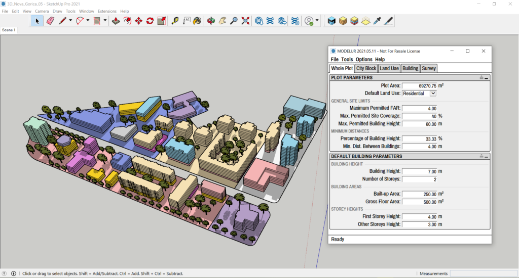
*The Excel Sample Spreadsheet is accompanied by a sample SketchUp file (.skp) that encompasses a 3D model of an urban development project. The data in an Excel sample spreadsheet is exported directly from that same project, using Modelur so LiveSync is already enabled.
To get free use case sample model skp. file, please write to us on info@modelur.com!

5 Excel Functions for Urban Designers and Architects
OFFSET
In the attached Excel Sample Spreadsheet, the OFFSET function is used to define the cell or range of cells that carry specific project data (for example Data on urban parameters of the City Blocks).
The purpose of the OFFSET function is to return a range that is a specified number of rows and columns from a reference cell or range. The range that the OFFSET function returns can be a single cell or a range of multiple adjacent cells.
The OFFSET function is meant to define a range that can be used in other formulas. You can use the OFFSET function to generate a range that expands and contracts by adjusting height and width.
Syntax: =OFFSET(reference, rows, cols, [height], [width])
Example: =OFFSET(cb_start,2,4)
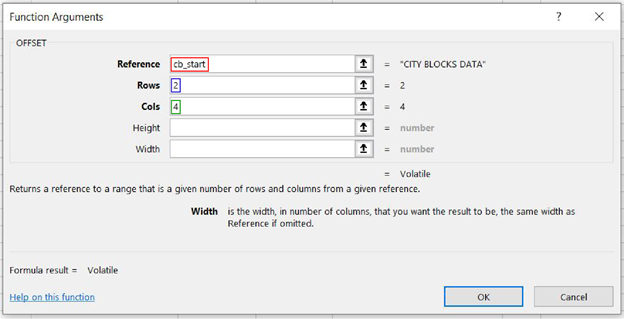
The first argument in OFFSET represents the first cell in the data (reference). Reference is the starting point from which you base the offset. The next two arguments are offsets for rows and columns.
VLOOKUP
VLOOKUPs’ abilities can be used to assess the environmental impacts of the developing project. For instance, CO2 impact can be assessed, having the default values of CO2 emissions for various building uses, specified regarding the year in which the buildings were constructed. Similarly, other important environmental impacts, such as water and electricity demand, can be assessed. Those calculations show us the current situation and predict the efficiency and performance of the plan.
One of the basic energy-related assessments is the factor of Energy Use Intensity (EUI). The attached Excel Sample Spreadsheet includes a use case of the average Energy Use Intensity (EUI) estimate for each building use on the urban design project development site.
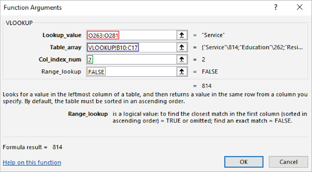
VLOOKUP is one of Excel’s most useful functions. It enables searching for values based on certain criteria (=other values). Those other values can be located in another part of the worksheet or a completely different worksheet. To use the VLOOKUP formula, you need to specify: the Lookup value (the key-value), the Table array (the range of values you want to search), and the column index number (column number) of the value you want to return.
Syntax: =VLOOKUP(lookup_value; table_array; col_index_num; [range_lookup])
Example: =VLOOKUP(C21:C38;B9:C16;2;FALSE)
MIN and MAX
MIN and MAX are simple functions useful in calculations examining some characteristics of planned development. For instance, in the sample spreadsheet we used MIN and MAX to find the smallest/largest city block or smallest/largest building floor area of the urban design project.
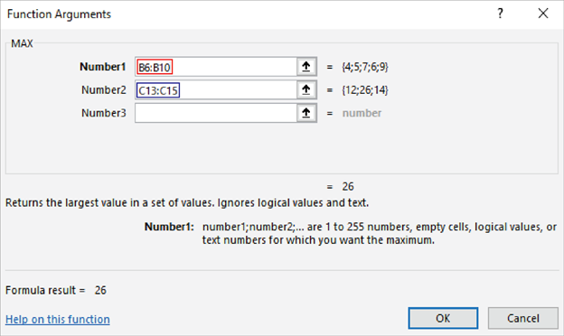
MIN returns the smallest number in the specified range of cells. MAX returns the largest number in a range of cells.
Syntax: =MIN(Number1;[Number2]; …) and =MAX(Number1;[Number2]; …)
Example: =MAX(B6:B10, C13:C15)
COUNTIF and COUNTIFS
COUNTIF(S) is a function to count cells in a range that meet specific criteria or conditions. When using the COUNTIF(S) function, only the data of specific city blocks or buildings meeting certain characteristics can be analyzed. For example, counting the buildings that have more than 30 residents or counting the buildings of each defined building use (E.g., Residential, School, etc.) on the development site.
Not dissimilar to COUNT (which counts the number of items in the specified range), the COUNTIF operator counts only instances that meet the single specified criteria. If you want to specify multiple criteria, use the COUNTIFS function instead.
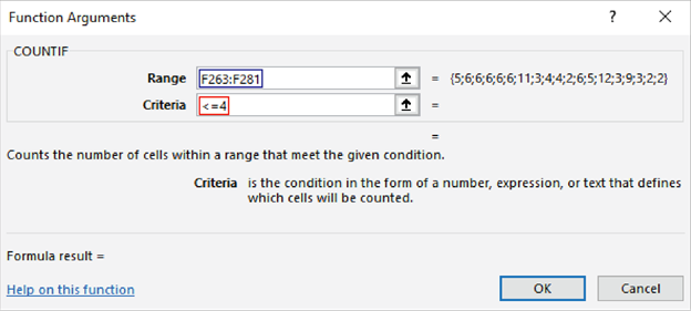
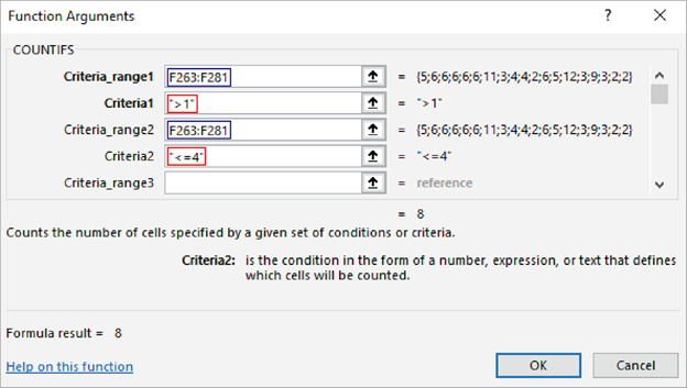
In the sample spreadsheet, COUNTIF and COUNTIFS function are used in a simple building height analysis. It counts the buildings that fall into one of the following categories: 1 storey; or more than 1 storey, but less or equal to 4 storeys; or 5 and more storeys. The information on the number of storeys is for example needed to make various decisions in planning the building’s elevators.
Syntax: =COUNTIF(criteria_range; criteria),
=COUNTIFS(criteria_range1; criteria1; criteria_range2; criteria2…)
Example: =COUNTIF(F263:F281;“<=4”)
Example: =COUNTIFS(F263:F281;“<=4“)
PIVOT TABLE
Pivot tables are useful in summarizing the large amounts of data on an urban design project. Series of tables can create numerous insights, from generating area totals (e.g., by city block, by buildings of various uses, by room type), to modeling the future economic impacts of varied planning provisions.
In the Excel Sample Spreadsheet, there are two Pivot Table use cases. In the first one, the Pivot Table creates an overview of the City Blocks and Buildings of the project site. The second use case is using a Pivot Table to display the exact number of Primary Units (e.g. Apartments, Offices) and Secondary Units (e.g. Residents, Employees) of each selected City Block on the project site.
The Pivot table is one of Excel’s most powerful built-in features. It automatically summarizes the data in a specified worksheet, so it can be “sliced and diced” in numerous ways. Furthermore, it provides a variety of ways to visualize the data.
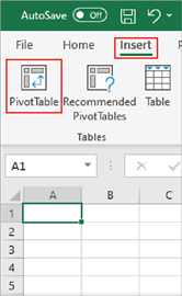
In the Excel file and worksheet with the data, you want to summarize, click Insert on the top menu, and click the “Pivot Table” icon.
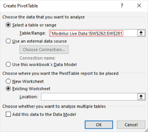
In the “Create PivotTable” dialog box, select the table or range (range of cells, containing the data that you want to summarize). Example of a data range specified: ‘Modelur Live Data’!$W$262:$W$281
You can also create Pivot Tables using external data sources such as databases. Once you’ve specified the range of data, choose where you want the Pivot Table to be placed. It can either place it in the current worksheet or a new worksheet. Click OK to insert the Pivot Table.
In the “PivotTable Fields” dialog, select the fields you want to be displayed in the Pivot Table. You can organize the Pivot table fields data in Rows, Values, Columns, and Filters.
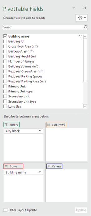
If you want to drill down on a particular value of the Pivot Table, double-click the value in the table. Excel will create a new worksheet with the corresponding data.
Updating the Pivot Tables
If you change the original data that a Pivot table contains, you’ll need to manually refresh it since Pivot Tables do not maintain a live link with the data. To refresh the Pivot table, select the table and navigate to the “Refresh” button in the “PivotTable Analyze” context ribbon (as seen in the image below).

Visualizing Pivot Table Data
In addition to viewing the data as a table, you can create Pivot table chart views. You can do so by selecting a Pivot Table and clicking the “Pivot Table Analyze” ribbon, then the “PivotChart” icon. In the “Insert Chart” dialog, choose the chart type, click “OK”, and the chart will be inserted on the same worksheet as the Pivot Table. Since the chart is linked to the Pivot Table data, it will update automatically once the Pivot Table is refreshed.

Inserting Pivot Table Slicers
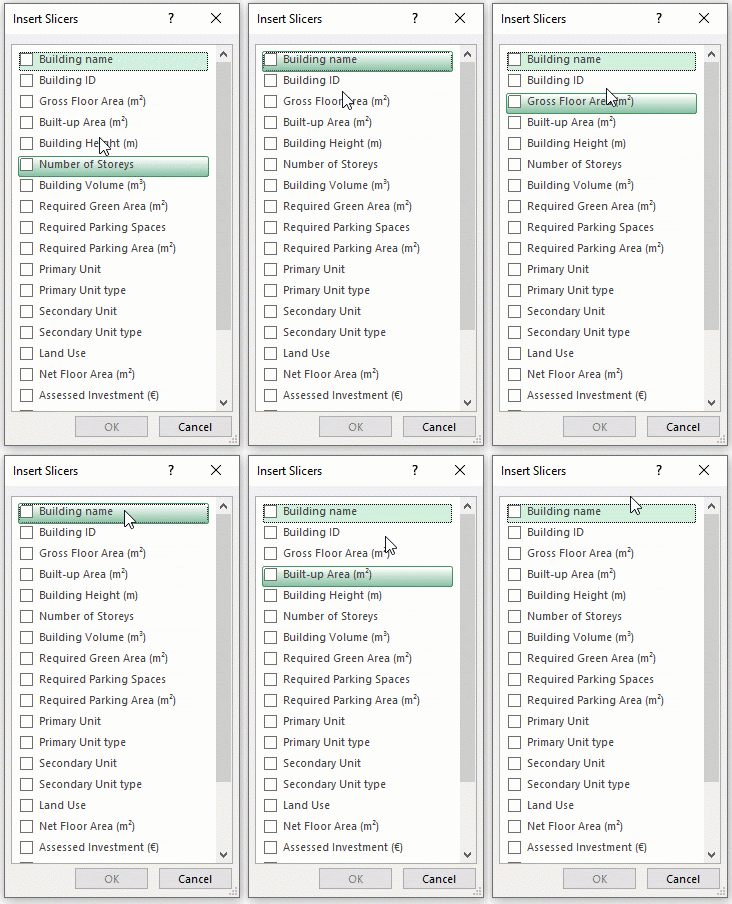
Pivot Table Slicers are a visual filter in the form of an interactive button, providing a dynamic way to graphically filter the Pivot Table data. To create a Slicer, select the Pivot Table and click on the “Insert Slicer” icon in the “PivotTable Analyze”. Choose the fields you want to “slice” and click OK to create a Slicer graphic object. If you click any value in the slicer graphic object, it filters the Pivot Table and any associated Pivot Charts accordingly. Pivot Slicers can be customized and connected to multiple Pivot Tables.

Work Faster with Modelur’s LiveSync for Excel
While a well-designed and comprehensive database is extremely helpful, manually creating the data to populate your database can be difficult. Every item must be entered individually, which can be tedious and error prone.
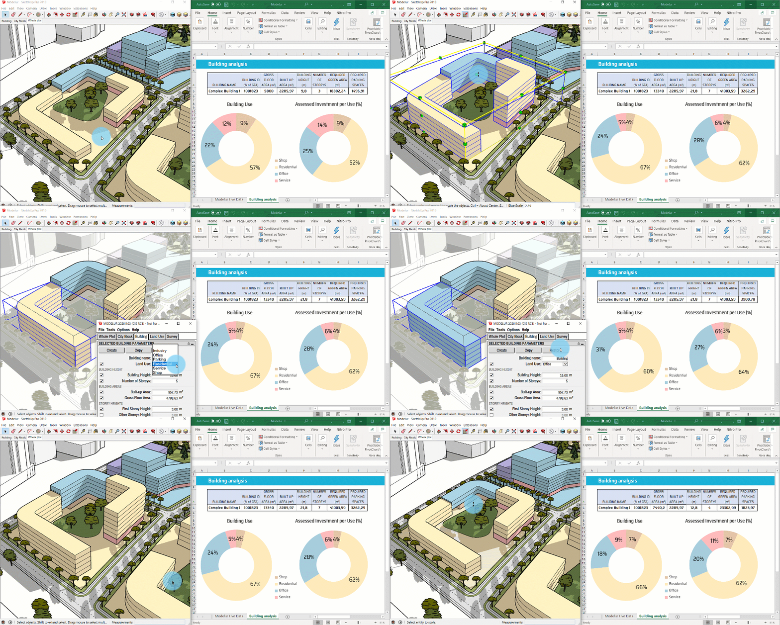
Fortunately, it is possible to skip this step entirely when using the Modelur plugin for SketchUp and Rhino. Data can be exported directly from the software its being designed on and saved to an Excel file that is ensured with LiveSync.
LiveSync to Excel enables you to export key urban performance indicators of your proposed development, including gross floor area, net floor area, built-up area, site coverage, floor area ratio, required parking lots, number of apartments, and many more. If any part of the development is later modified, LiveSync with Excel updates the data instantly. This feature enables you to track key performance indicators for urban growth and development for status and progress discussions with stakeholders such as the city council and development organizations.
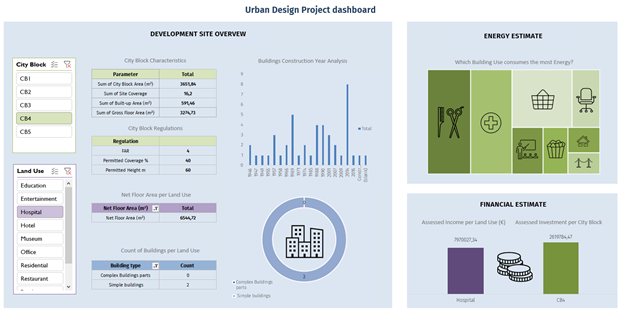
Another great feature of Excel that urban designers and architects should be familiar with is dynamic dashboards. These dashboards are a visually appealing and easy way to summarize KPIs, key urban parameters, characteristics of a project, and more. These dashboards can be made of tables, charges, gauges, etc. depending on the needs of the project or to whom you are presenting.
Their benefit lies in the ability to simplify complex data and provide an at-a-glace view of a project in real-time. Therefore, even a simple dashboard can offer a high-level view of work, helping urban designers and architects to communicate their projects to the stakeholders and make quick decisions.
Dynamic Dashboards can be created with a simple data set but are best achieved when utilizing pivot tables as discussed above. These pivot tables will allow for not just a visual representation, but also calculations of the data. An example of an Urban Design Project Dashboard:
This was only a glimpse into the possibilities of using Excel to accelerate your work process while reducing errors. Be sure to download our sample spreadsheet so that you can see how each function listed above works as well as how Modelur’s data can be used in your projects.
We recommend checking out this great series of short articles on Excel for Architects if you are looking to learn more.
Do you find this article useful? You are invited to share your favorite Excel functions, tips, tricks, and thoughts below in the comments! You can follow our Linkedin page so you don’t miss further content. Stay tuned and thank you!


